4.1. Styles

4.1.1. CLIP_GAUGE

Used to clip model input grids to the spatial extent of the digital elevation model (DEM) defined in the Basic block.

OUTPUT GRIDS

maskgrid.tif: Binary mask grid that covers the entire spatial extent of the DEM.

Example of a basin mask .tif file generated using the CLIP_GAUGE task style.

basin_new.txt: Text file containing the gauges and basin to cover the entire DEM domain

[Gauge 0] cellx=7198 celly=10880 outputts=false #Num Cells = 48893468.000000
[Gauge 1] cellx=2180 celly=9025 outputts=false #Num Cells = 6793795.000000
...
[Basin 0]
gauge=0 gauge=1 ...

Example of CLIP_GAUGE control file

...

 [Task CLIPGAGING]
 STYLE=CLIP_GAUGE
 MODEL=crest
 ROUTING=KW
 BASIN=0
 PRECIP=IMERG
 PET=CLIMO
 OUTPUT=outputs
 defaultparamsgauge=0
 PARAM_SET=MyCRESTPAR_90
 ROUTING_PARAM_Set=MyKWPAR_90
 TIMESTEP=30u
 TIME_BEGIN=202010100830
 TIME_END=202010100930

4.1.2. BASIN_AVG

EF5 supports spatial aggregation of input grids. The aggregation is computed by averaging the accumulated values of the variable by the flow accumulation grid. The output grid corresponds to the average value of the variable in each catchment area. To run the aggregation task, set the STYLE parameter in the Task block to BASIN_AVG. The variables to be averaged should be located inside the output folder defined in the Task block. The aggregation will be performed for all the variables (.tif) found in the output folder. The aggregation zone is defined by the most downstream gauge in the BASIN block. If the user requires to be computed for the entire domain, the CLIP_GAUGE task style can be used to automatically identify all outlets and create a basin that covers the entire domain. The following output grids will be generated in the output folder:

OUTPUT GRIDS

basin.area.tif: Catchment area at each pixel (km²).

relief.ratio.tif: Relief ratio at each pixel (m/km).

relief.tif: Relief at each pixel (m).

river.length.tif: Length of the river network at each pixel (km).

your_variable_1.tif.avg.tif: Average of the variable “1” in each pixel.

your_variable_2.tif.avg.tif: Average of the variable “2” in each pixel.

...: Additional variables processed if tif located in the outputs folder.

Example of BASIN_AVG control file

...

 [Task BASINAVGING]
 STYLE=BASIN_AVG
 MODEL=crest
 ROUTING=KW
 BASIN=0
 PRECIP=IMERG
 PET=CLIMO
 OUTPUT=outputs
 defaultparamsgauge=0
 PARAM_SET=MyCRESTPAR_90
 ROUTING_PARAM_Set=MyKWPAR_90
 TIMESTEP=30u
 TIME_BEGIN=202010100830
 TIME_END=202010100930

4.1.3. SIMU using long range mode

The Long Range mode enables EF5 to incorporate forecasted precipitation datasets in addition to the standard observed precipitation inputs. This is particularly useful for generating forecast simulations beyond the observation window.

To activate Long Range mode, configure the Task block as follows:

Set the STYLE parameter in the Task block to SIMU
Provide both, the PRECIP and the PRECIPFORECAST parameter with the name of the precipitation forecast block defined in the control file.

...

 [Task Simulation_QPF]
 STYLE=SIMU
 MODEL=crest
 ROUTING=KW
 BASIN=0
 PRECIP=IMERG                        # Observed precipitation forcing
 PRECIPFORECAST=GFS                  # Precipitation forecast forcing
 PET=CLIMO
 OUTPUT=outputs
 STATES=states
 OUTPUT_GRIDS=MAXUNITSTREAMFLOW|MAXSTREAMFLOW|PRECIPACCUM
 defaultparamsgauge=0
 PARAM_SET=MyCRESTPAR
 ROUTING_PARAM_Set=MyKWPAR
 TIMESTEP=30u
 TIME_BEGIN=202001010000
 TIME_WARMEND=202002010000
 TIME_STATE=202003010000
 TIMESTEP_LR=60u                     # Time step for long range mode
 TIME_BEGIN_LR=202003010000          # Start date for forecast forcing
 TIME_END=202003011200               # End date of simulation including forecast period

4.1.4. DATA ASSIMILATION

EF5 supports data assimilation (DA) of streamflow observations to improve hydrologic simulations. The DA process adjusts model states based on observed streamflow data at specified gauge locations. The following figure illustrates the effect of data assimilation on streamflow simulations.

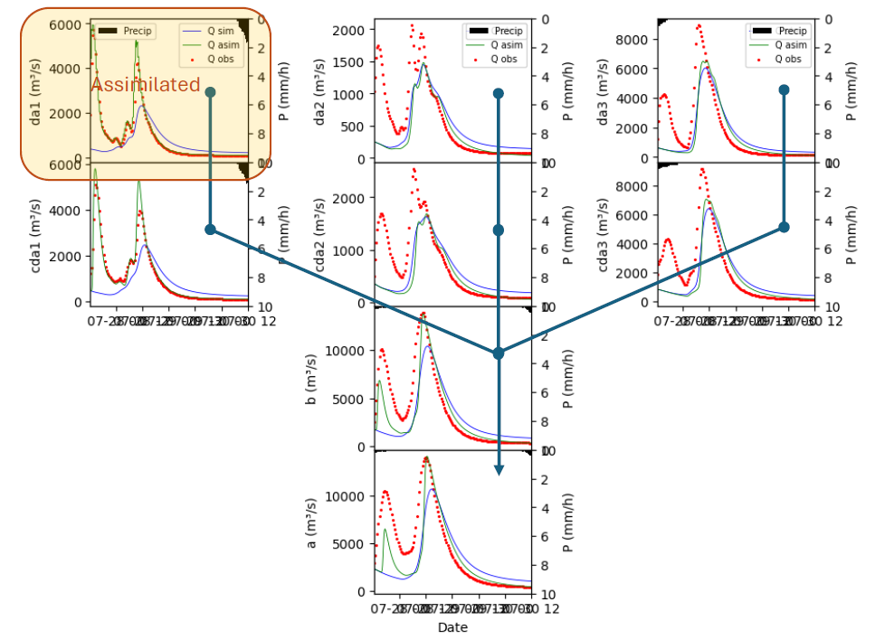
_images/da_effects.png — Example of the effect of data assimilation on streamflow simulations using EF5. The blue line represents the simulated streamflow without data assimilation, while the green line shows the improved simulation after assimilating observed data (red dots).

EF5 requires the user to provide a file containing streamflow observations for the gauges defined in the BASIN block. The file should be in CSV format with the following structure (no header):

da1,2022-07-27 12:30:00,1924.11
da1,2022-07-27 13:00:00,4197.91
...

da2,2022-07-27 12:30:00,1030.03
da2,2022-07-27 13:00:00,1255.62
...

Example of Data Assimilation control file:

...

[gauge A] lat=37.755 lon=-84.025 outputts=true
[gauge DA1] lat=37.384 lon=-83.684 outputts=true WANTDA=true OBS=obs/DA1.csv   # Enable data assimilation for this gauge
[gauge DA2] lat=37.443 lon=-83.464 outputts=true WANTDA=true OBS=obs/DA2.csv   # Enable data assimilation for this gauge

[Basin 0]
gauge=A
gauge=DA1
gauge=DA2

...

[Task CREST_Simulation]
STYLE=simu
MODEL=crest
ROUTING=KW
BASIN=0
PRECIP=MRMS
PET=CLIMO
OUTPUT=outputs
STATES=data/states
DA_FILE=da.observations.csv # Name of the file containing streamflow observations for data assimilation
defaultparamsgauge=A
...

[Execute]
task=CREST_Simulation

Warning

🚧 This documentation is currently under active development. Content may change frequently and some sections may be incomplete.